A step by step guide on how to collect and preprocess satellite imagery data for machine learning algorithms
This article is the first part of a 2 part series which explores the uses of machine learning algorithms on satellite imagery. Here we will focus on the data collection and preprocessing steps while the second part will showcase the use of various machine learning algorithms.
TL;DR
This article will:
We will use the detection and classification of agriculture fields as an example. Python and jupyter notebook are used for the preprocessing steps. The jupyter notebook for reproducing the steps is available in github.
This article assumes basic fundamentals in data science and python.
Computer vision is a fascinating branch of machine learning that has been quickly developing in past years. With public access to many off the shelf algorithm libraries (Tensorflow, OpenCv, Pytorch, Fastai …) as well as open source datasets (CIFAR -10, Imagenet, IMDB …) it’s very easy for a data scientist to get hands on experience on this topic.
But did you know that you could also access open source satellite imagery ? Those types of imagery can be used in a wealth of use cases (Agriculture, Logistics, Energy …). However, they provide additional challenges for a data scientist due to their size and complexity. I have written this article to share some of my key learnings working with them.
Step 1 — Select the satellite open data source
First, you need to choose which satellite you want to use. Key features to watch out for here are :
Here are satellites whose data are available free of charge :
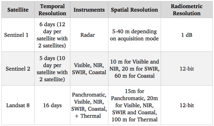
Benchmark of satellite systems
Since our goal is to detect and identify agricultural crops, the visible spectrum (which is used to provide standard color images) should be quite useful. Additionally there are correlations between nitrogen level of crops and NIR (Near-infrared) spectral bands. As far as free options go, Sentinel 2 is currently the best in terms of resolution with 10 m for those spectral bands, so we are going to use this satellite.
Of course, 10 m resolution is much lower compared to state of the art in satellite imagery with commercial satellites reaching a 30 cm resolution. Access to commercial satellite data can unlock many use cases, but despite increasing competition with new players entering this market, they remain highly priced and hence difficult to integrate in a scaled use case.
Step 2 — Collect the satellite imagery data from Sentinel 2
Now that we have selected our satellite source, the new step is to download the images. Sentinel 2 is part of the Copernicus Programme from the European Space Agency. We can access its data using the SentinelSat python API.
We first need to create an account at the Copernicus Open Access Hub. Alternatively note that this website also provides a way to query images with a GUI.
A way to specify the zones you want to explore is to provide the API with a geojson file, which is a json containing GPS coordinates position (latitude and longitude) of a zone. Geojson can be quickly created on this website.
This way you can query all the Satellite images intersecting with the zone provided.
Here we list all images available on a for a given zone and time range :
api = SentinelAPI(
credentials[“username”],
credentials[“password”],
“https://scihub.copernicus.eu/dhus”
)
shape = geojson_to_wkt(read_geojson(geojson_path))
images = api.query(
shape,
date=(date(2020, 5, 1), date(2020, 5, 10)),
platformname=”Sentinel-2″,
processinglevel = “Level-2A”,
cloudcoverpercentage=(0, 30)
)
images_df = api.to_dataframe(images)
Note the use of arguments:

images_df
Images_df is a pandas dataframe containing all images that match our query. We select one with a low cloud cover and download it using the api :
api.download(uuid)
Step 3 — Understand which spectral bands to use and manage quantization
Once the zip file is downloaded we can see that it actually contains several images.
This is because as we said in step 1, Sentinel 2 captures many spectral bands and not only Red Green and Blue and each band is captured in a single image.
Also its instruments do not all have the same spatial resolution, so there is a subfolder for each different resolution 10, 20 and 60 meters.
If we check the GRANULE/<image_id>/IMG_DATA folder we see that there is a subfolder for each different resolution: 10, 20 and 60 meters as the spectral bands. We are going to use those with max resolution 10m as they provide Band 2, 3, 4 and 8 which are Blue, Green, Red and NIR. Band 7, 8, 9 which are vegetation red edge (spectral bands between red and NIR that mark a transition in reflectance value for vegetation) could also be interesting for detecting crops but since they are lower resolution we are going to leave them aside now
Here we load each band as a 2D numpy matrix:
def get_band(image_folder, band, resolution=10):
subfolder = [f for f in os.listdir(image_folder + “/GRANULE”) if f[0] == “L”][0]
image_folder_path = f”{image_folder}/GRANULE/{subfolder}/IMG_DATA/R{resolution}m”
image_files = [im for im in os.listdir(image_folder_path) if im[-4:] == “.jp2”]
selected_file = [im for im in image_files if im.split(“_”)[2] == band][0]
with rasterio.open(f”{image_folder_path}/{selected_file}”) as infile:
img = infile.read(1)
return img
band_dict = {}
for band in [“B02”, “B03”, “B04”, “B08”]:
band_dict[band] = get_band(image_folder, band, 10)
A quick test to make sure everything is working is trying to recreate the true color image (ie RGB) and display it using opencv and matplotlib:
img = cv2.merge((band_dict[“B04”], band_dict[“B03”], band_dict[“B02”]))
plt.imshow(img)
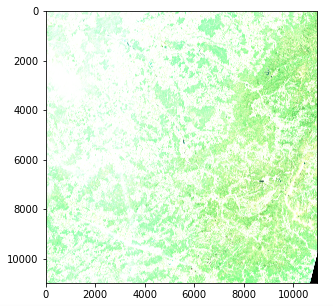
Satellite Image — Color intensity issue (Copernicus Sentinel data 2020)
However there is an issue with color intensity. This is because the quantization (number of possible values) differs from the standard for matplotlib which assumes either a 0–255 int value or a 0–1 float value. Standard images often use an 8 bit quantization (256 possible values) but Sentinel 2 images use a 12 bit quantization and a reprocessing converts the values to a 16 bit integer (65536 values).
If we want to scale a 16 bit integer to an 8 bit integer we should in theory divide by 256 but this actually results in a very dark image since the whole range of possible values is not used. The max value in our image is actually 16752 out of 65536 and few pixels actually reach values higher than 4000 so dividing by 8 actually gives an image with a decent contrast
img_processed = img / 8
img_processed = img_processed.astype(int)
plt.imshow(img_processed)
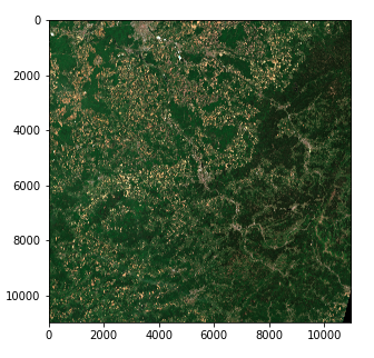
Satellite Image — Right color intensity (Copernicus Sentinel data 2020)
We now have a 3 dimension tensor of shape (10980, 10980, 3) of 8 bit integers in the form of a numpy array
Note that :
Step 4 — Split the images to machine learning ready sizes
We could try applying an algorithm to our current image but in practice that would not work with most techniques due to its size. Even with strong computing power, most algorithms (and especially deep learning) would be off the table.
So we must split the image into fragments. One question is how to set the fragment’s size.
We decide to go for splitting each image in a 45 * 45 grid (45 being conveniently a divider of 10980)
Past this parameter fixing, this step is straightforward using numpy array manipulation . We store our values in a dict using (x, y) tuples as keys.
frag_count = 45
frag_size = int(img_processed.shape[0] / frag_count)
frag_dict = {}
for y, x in itertools.product(range(frag_count), range(frag_count)):
frag_dict[(x, y)] = img_processed[y*frag_size: (y+1)*frag_size,
x*frag_size: (x+1)*frag_size, :]
plt.imshow(frag_dict[(10, 10)])
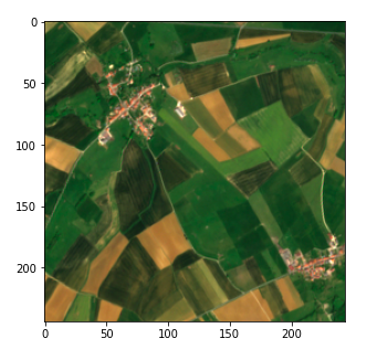
Fragment of the satellite image (Copernicus Sentinel data 2020)
Step 5 — Link your data to the satellite images using GPS to UTM conversion
Finally we need to link our images with the data we have on agricultural fields to enable a supervised machine learning approach. In our case we have data on agricultural fields in the form of a list of GPS coordinates (latitude, longitude) , similar to the geojson we used in step 2 and we want to be able to find their pixel position. However, for the sake of clarity, I will start by showcasing a pixel conversion to GPS coordinates and then show the reverse
The metadata collected while requesting the SentinelSat API provides the GPS coordinates of the corners of the image (footprint column) and we want the coordinates of a specific pixels. Latitude and longitude which are angular values do not evolve linearly within an image so we cannot do a simple ratio using the pixel position. There are ways to solve this using math equations but off the shelf solutions already exist in python.
One quick solution is to convert the pixel position to UTM (Universal Transverse Mercator) in which a position is defined by a zone as well as an (x, y) position (in meter unit) which does evolve linearly with the image. We can then use a UTM to Latitude / Longitude conversion provided in the utm library. To do this we first need to obtain the UTM zone and position of the upper left corner of the image which can be found in true color image’s metadata.
#Obtaining meatadata
transform = rasterio.open(tci_file_path, driver=’JP2OpenJPEG’).transform
zone_number = int(tci_file_path.split(“/”)[-1][1:3])
zone_letter = tci_file_path.split(“/”)[-1][0]
utm_x, utm_y = transform[2], transform[5]
# Converting pixel position to utm
east = utm_x + pixel_column * 10
north = utm_y + pixel_row * – 10
# Converting UTM to latitude and longitude
latitude, longitude = utm.to_latlon(east, north, zone_number, zone_letter)
The GPS position to pixel conversion is done using the reverse formulas. In that case we have to make sure that the zone obtained matches with our image. This can be done by specifying the zone. If our object is not present in the image this will result in an out of bound pixel value.
# Converting latitude and longitude to UTM
east, north, zone_number, zone_letter = utm.from_latlon(
latitude, longitude, force_zone_number=zone_number
)
# Converting UTM to column and row
pixe_column = round((east – utm_x) / 10)
pixel_row = round((north – utm_y) / -10)
view raw
Conclusion
We are now ready to use the satellite images for machine learning !
In the next article of this 2 part series we will see how we can use those images to detect and classify fields surfaces using both supervised and unsupervised machine learning.
Thanks for reading and don’t hesitate to follow the Artefact tech blog if you wish to be notified when this next article releases !

 BLOG
BLOG