
NEWS / AI TECHNOLOGY
25 november 2020
At Artefact, we are so French that we have decided to apply Machine Learning to croissants. This first article out of two explains how we have decided to use Catboost to predict the sales of “viennoiseries”. The most important features driving sales were the last weekly sales, whether the product is in promotion or not and its price. We will present to you some nice feature engineering including cannibalisation and why you sometimes need to update your target variable.
What is it?
At Artefact, we are so French that we have decided to apply Machine Learning to croissants. This first article out of two explains how we have decided to use Catboost to predict the sales of “viennoiseries”. The most important features driving sales were the last weekly sales, whether the product is in promotion or not and its price.
We will present to you some nice feature engineering including cannibalisation and why you sometimes need to update your target variable. We chose the Forecast Accuracy and the biais as evaluation metrics. Our second article will explain how we put this model in production and some best practices of ML Ops.
For who?
- Data Scientist, ML Engineer or Data lovers
Takeaways?
- Boosting algorithms for time series prediction
- How to answer a forecasting problem with noisy data
- How to handle operational constraints in production
Context
We have been recently working on a really interesting and challenging topic for a huge retailer in France: How to predict the daily demand of fresh perishable products such as pastries, including our beloved croissants.
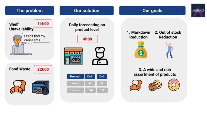
This retailer was facing a classic problem of supply chain: each day their bakers have to bake a certain amount of fresh, perishable products: croissants, chocolate breads, baguettes, lemon pies etc. Most of these products don’t last more than one day, if they are not sold they are considered as lost revenue. On the other hand if there is unavailability on-shelf during the day, it will lead to unhappy consumers and a loss of money. The challenge is to predict on a daily level, seven days in advance the amount of each perishable product for each store. As a result, this project aimed to improve shelf availability while reducing food waste.
To predict sales a few days in advance, an internal solution using simple statistical measures was already used. Yet, after meeting the bakery managers, we understood that there was a clear room for improvement leveraging more data and features such as seasonality effects, weather, holidays, product substitution effects, etc. We have thus decided to use the current solution as baseline and try more recent algorithms to improve the forecast accuracy.
And to conclude this introduction, an illustration of the challenge and what we want to achieve.
Model development
Now that we have a well defined problem and some goals to achieve, we can finally start writing some nice python code in our notebooks — let the fun begin!
Data request
As in any data science project, it all starts with data. From experience we strongly recommend asking for the data request as soon as possible. Don’t be shy to ask for a lot of data and for each data source be sure to identify a referent, someone you can easily contact and ask your questions about the data collection or how the data is structured.
Thanks to the different meetings we were able to draw a list of the data we could use:
- Transactional data including price of products.
- Promotions: a list of all the future promotions and their associated prices.
- Product information: different characteristics related to the products.
- Store information: location, size of the stores, competitors.
- Weather data.
- Waste data: at the end of each day, how many products were thrown away.
Exploratory Data Analysis (EDA) and outliers detection
Once the data was collected, we started to do some analysis. Is there seasonality in my data? A trend? How many products do I have? Are they consistent over time? Are there seasonal products?
By plotting the different time series, we also spotted some interesting features:
- Seasonality over the year but also during the week.
- Pricing and if the product is in promo or not.
- Cannibalisation of products and deferred sales during out of stock.
- Sales pattern differing from one store to another.
Note that we created different features related to the pricing. The absolute price but also the relative prices compared to other products in the same subfamily, family or store. The relative price is one way to quantify price cannibalisation between products. We also created features translating the price variation of one product over time.
For such down to earth prediction tasks, devils are in the details and it is really important to look for outliers and anomalies, to take the time to crunch your data.
But first, why should we even bother with outlier detection? Many reasons, it may indicate bad data, mistakes in the ETLs, business processes you didn’t know. Secondly it is really likely that it will impact your algorithm and the inference part so it is definitely an important part of development.
You can spot outliers at different times of the project, either during the exploratory data analysis (EDA) or by analysing the biggest errors of your models.
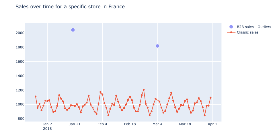
While doing the EDA, we spotted some strange data such as B2B sales, for instance 1800 sales of a single item on a single purchase receipt. Outliers related to the pricing, mostly due to manual mistakes by the cashier: negative prices or a croissant costing 250 euros!
We noticed that sometimes our predictions were totally off the first days of the promotion periods. After some analysis we noticed that it was due to the fact that the promotion was launched one day before or after the official day. Indeed sometimes the manager took some liberty and decided to change the beginning or the end of the promotions. These changes can be spotted and fixed in the training data set but can lead to big errors in prediction. Indeed promotions can reach volumes 4 to 5 times bigger than in non promotion.
Here a list of some other interesting examples of process and mechanisms we discovered thanks to this analysis and you may find in your projects:
- The assortment is not always consistent over days due to operational constraints, errors, stock management.
- For some data sources, the dates indicated were the days the data was loaded as a result you need to remove one day to get the real day.
From sales prediction to optimal sales prediction
A challenge led us to update our target variable. Sometimes due to an unexpected influence or bad forecasting, the department expected a shortage of products before the end of the day. Two phenomena can then happen: the customer not being able to find his product doesn’t buy anything, or buys a similar good. Based on historical data, we inferred some distribution laws (basic statistics) that helped us to modelise this impact and updated our target variable in order not to predict the historical sales but the optimal sales for a particular product.
This update of the target variable is tricky because it is really hard to know if the update made sense. Did you really improve the quality of the data or make it worse? One way to quantify our impact was to take sales without out of stock and create false shortage, for instance remove all sales after 5 or 6pm and then try to reconstruct the sales. This method helps us to get back to a classic supervised problem that we can assess objectively.
As a result we were able to predict the optimal sales and avoid our algorithm to learn shortage patterns.
Our models
After having properly cleaned our data we can finally test and try a few models.
You have a lot of different possibilities to address a forecasting problem: classical statistical approaches (SARIMA, Exponential Smoothing, Prophet, etc.), machine learning approaches (Linear Regression, Boosting Algorithms) or Deep Learning (RNN, LSTM, CNN). How to choose the right approach is a tricky question, here are some elements which helped us to choose:
- Not one but many time series: ~10 000
- Irregular time series: it can happen that there is no sales for some days due to manager choices, business or operational constraints.
- Promotions have a huge impact and are not seasonal or cyclic.
- We observed a huge correlation between sales at J-0 and the sales of at J-7, J-14, J-21 for items per store and the state of being in promotions or not.
- Exogenous data have an impact on the sales: prices, special days, etc.
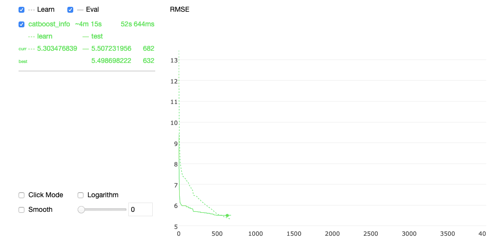
For these reasons, we decided to choose Catboost as a model. Catboost has a lot of advantages such as handling natively categorical and missing values, can handle a lot of features, scales well and can infer a lot of time series within the same model. Moreover it provides a nice plot while training and integrates really easily with SHAP for the feature importance.
Here for instance a screenshot of the interactive plot of the algorithm during its training:
Nevertheless, one of the drawbacks of pure ML approaches is the necessity of coding all the features yourself, especially the ones related to time. Without strong feature engineering these algorithms will be unable to catch the time patterns. Moreover they can only infer a fixed time frame unlike Sarima or Prophet where you can specify the number of days to forecast using the periods parameter.
Finally you have to be very careful with data leakage especially when you build your lag feature.
One of the main features was not the weekly lag but the average of the lags: D-7, D-14, D-21, … etc last six weeks. Indeed the non regular characteristic of our time series mixed with the use of promotion from time to time induce a fuzzy seasonality, hence the use of an average. It is important to notice that just using this average as a unique model already gives really good performance!
One model vs many models
To sum up we used one algorithm: Catboost, to predict all our 10 000 time series, for each product and each store. But what if an item has a really particular sales pattern, or a specific store? Would the algorithm identify and learn this pattern?
These questions lead us to the question, should we cluster our products, stores and train one algorithm per cluster? Even if the use of decision tree algorithms should tackle this challenge, we observed limitations in some specific cases.
Boosting algorithms are iterative algorithms, based on weak learners which will focus on their biggest errors. It is obviously a bit oversimplified but it helps me to point out one of their limitations. If you didn’t normalise your target variable, your algorithm will “only” focus on products with big errors which are to be more likely the one with the biggest sales. As a result, the algorithm may focus more on the products or stores with bigger sales volume.
We didn’t find the perfect way to address this challenge but we observed some improvements by clustering our products/stores by family or selling frequency.
One of the advantages of training multiple algorithms are:
- Quicker to train
- Easier to fine tune
- Easier to debug
- In case of data anomalies not all models will go wrong
- Depending of the products, you can play with the loss function and promote shortage or over production
But on the other hand, it will be more challenging to maintain!
In the end we decided to go with this approach as this was yielding better results.
How to evaluate our model?
We discussed a lot of models and their performances in the previous sections. But how does one evaluate a forecasting algorithm? Obviously it is really similar to any machine learning problems but nevertheless it has its own specificities:
- Cross Validation
As mentioned before, one of the challenges of time series forecasting is to avoid data leakage. It can happen while creating our features: lags, normalization of our variables, etc…
But it may also happen while doing cross validation, split between train, validation and test datasets.
You can’t use the classic train_test_split() from sklearn. Why? Imagine your dataset is the sales of 2019, if you split randomly, you will train on data from jan, feb, …, december 2019 and your test data will have sales from the same dates! As a result, your algorithm will train on patterns that he will not have in production hence a data leakage issue. To solve that there are other ways to split your data such as the function TimeSeriesSplit() also from sklearn.
2. The choice of the metric:
Time series forecasting is a regression problem, as a result we may use the classic metrics such as MSE, RMSE but others are also available, here a non exhaustive list:
- MAPE or Forecast Accuracy
- A weighted MAPE
- Dynamic Time Warping
We optimised our algorithm using RMSE, but to communicate with our business owners used a weighted Forecast Accuracy:

We calculated it first at a day/store level and then aggregated it by store using a weighted average, the weights being the sales per day of the different stores. This metric can obviously be challenged but it has the advantage of having a value for each store, and if one day the manager really outperforms (badly or well) it is not over estimated. Moreover FA is a really interpretable metric which speaks to the business unlike RMSE.
Finally another metric interesting to keep in mind is the biais, which introduces the overall trend of the algorithm to overpredict or underpredict. Depending on the business case you may want to push one or another. In our case we pushed a slight over prediction to be sure to have the product on the shelf and keep our customer happy!
Final words, some advice for any data projects
I thought it would be also nice to share with you some tips, mistakes we make on a project level.
First of all, how did we develop our models, feature engineering?
All these different steps, experiments were realized in notebooks, but the use of notebooks doesn’t mean dirty code! On the contrary, we highly recommend taking the time to write proper notebooks with titles, proper names, functions, and factorize redundant lines.
The use of notebooks brings up some challenges especially when many developers work together: conflicts on github, no replicable code, etc…
Here are some tips to reduce these problems:
- Version your notebooks using markdowns
- Avoid working together on the same notebooks
- If you still do, to handle conflicts in notebook use the nbdev library from fastai
- Package common functions into .py files as a result everyone will use the same ones
- To version your experiment use tools such as ML Flow
- Avoid print() and use a logger instead, only log useful information. Check out scikit-lego which has pretty cool features, decorators.
- If you really want to print things try the library rich which makes it nicer and can also be used as a logging tool. Here a quick demo of rich by calmcode.io
Key Takeaways
We would have loved to share with you our results but we were not allowed due to privacy reasons but we can say that with these methodology we were able to:
- Be as good as their best demand planner
- Increase the FA of some store up to 30%
But on the other hand, here the list of our biggest learnings that I hope will help you to develop your own solution:
- Take the time to understand your problem, define a clear measurable objective, evaluation metric
- Crunch and explore your data, if you didn’t find anomalies… you didn’t look enough!
- Track rigorously your experiments
- Write clean code especially in notebooks, it will make your life so much easier for deployment
- Always think production, data leakage are your worst enemy in time series forecasting
- Start with a small scope, with simple models, test, fail, learn, improve and succeed!

 BLOG
BLOG


