

Author


Assortment optimization is a critical process in retail that involves curating the ideal mix of products to meet consumer demand while taking into account the many logistics constraints involved. The retailers need to make sure that they offer the right products, in the right quantities, at the right time. By leveraging data and consumer insights, retailers can make informed decisions on which items to stock, how to manage inventory, and what products to prioritize based on customer preferences, seasonal trends, and sales patterns.
For retail businesses, assortment optimization is essential to striking a balance between variety and efficiency. Offering too few choices may drive customers away, while offering too many can lead to confusion, excess inventory, and lower profit margins. Optimizing the product assortment helps businesses enhance customer satisfaction by ensuring popular items are available while eliminating underperforming products that take up valuable shelf space.
Choice modeling is an efficient way to approach assortment optimization because it provides a data-driven framework for understanding customer preferences and predicting how they will choose between different products. By analyzing various factors such as price sensitivity, product features, and brand loyalty, choice modeling helps retailers identify which products are most likely to meet customer demand.
Ultimately, choice modeling enables retailers to offer the right mix of products, tailor assortments to specific customer segments, and can also optimize shelf space to drive profitability or even the pricing of items.
If you have never heard of choice modeling, you can read our article that introduces the key concepts with examples. In this article, we will mainly focus on how discrete choice models can be used to optimize an assortment of products. We provide code samples based on the choice-learn library, which is designed to help data scientists on such use cases.
The provided code uses the choice-learn Python package and can be found in a notebook here.
Set up: Installing Python & Choice-Learn
In this article, we provide code snippets to accompany the explanations. The code uses the Choice-Learn library, which provides efficient tools for choice modeling and several applications — such as assortment optimization or price. Choice-Learn is available through PyPI, you can get it simply with
The dataset : sales receipts
We will use the TaFeng grocery dataset. You can download it from Kaggle and open it in your Python environment with choice-learn:
print(tafeng_df.head())
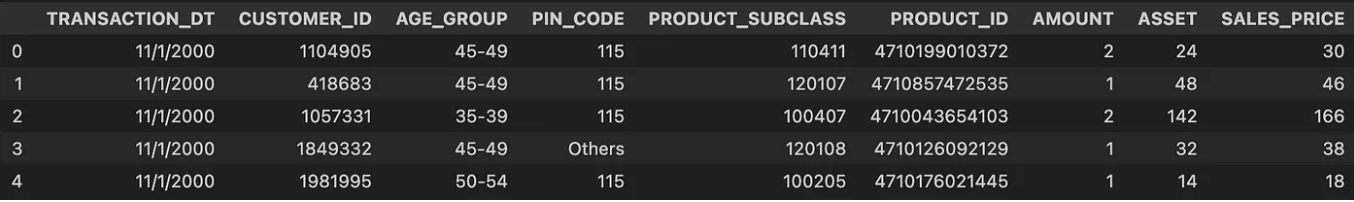
The dataset consists of over 800,000 individual purchases in a Chinese grocery store. For each purchase, various details are provided, including the purchased item (PRODUCT_ID), the price at which it was sold (SALES_PRICE), and the customer’s age group (AGE_GROUP).
You can observe that many different items are provided and some of them are seldom sold. In order to streamline logistics, the retailer may choose to reduce the number of products they offer. The goal in this case is to identify the optimal subset of items to sell.
To achieve this, we focus on the top-selling items, as they are more likely to be purchased again and will play a crucial role in shaping a more efficient and profitable assortment. Note that we do this mainly to simplify the example and that all items could be kept.
tafeng_df = tafeng_df.loc[
tafeng_df.PRODUCT_ID.isin(tafeng_df.PRODUCT_ID.value_counts().index[:20])
].reset_index(drop=True)
tafeng_df = tafeng_df.loc[
tafeng_df.AGE_GROUP.isin([“25-29”, “40-44”, “45-49”, “>65”, “30-34”, “35-39”, “50-54”, “55-59”, “60-64”] )
].reset_index(drop=True)
Let’s also encode the age categories with one hot values every ten year:
tafeng_df[“twenties”] = tafeng_df.apply(lambda row: 1 if row[“AGE_GROUP”] == “25-29” else 0, axis=1)
tafeng_df[“thirties”] = tafeng_df.apply(
lambda row: 1 if row[“AGE_GROUP”] in ([“30-34”, “35-39”]) else 0, axis=1
)
tafeng_df[“forties”] = tafeng_df.apply(
lambda row: 1 if row[“AGE_GROUP”] in ([“40-44”, “45-49”]) else 0, axis=1
)
tafeng_df[“fifties”] = tafeng_df.apply(
lambda row: 1 if row[“AGE_GROUP”] in ([“50-54”, “55-59”]) else 0, axis=1
)
tafeng_df[“sixties_and_above”] = tafeng_df.apply(
lambda row: 1 if row[“AGE_GROUP”] in ([“60-64”, “>65”]) else 0, axis=1
)
Now that our data is ready, we need to create a ChoiceDataset, the data handler object in choice-learn. This involves specifying the features that describe the context in which a purchase is made:
- Customer characteristics (shared features): the age category
- Product characteristics (item features): the item price
A key aspect of choice modeling is that we require the characteristics of all available items at the time of a purchase, not just the chosen one. This allows us to analyze how the prices of different products influence the customer’s decision. Since this information isn’t directly available in the dataset, we make the assumption that for each purchase, the prices of the other items remain the same as they were in the previous sale.
id_to_index =
for i, product_id in enumerate(np.sort(tafeng_df.PRODUCT_ID.unique())):
id_to_index[product_id] = i
# Initialize the items price
prices = [[0] for _ in range(len(id_to_index))] for k, v in id_to_index.items():
prices[v][0] = tafeng_df.loc[tafeng_df.PRODUCT_ID == k].SALES_PRICE.to_numpy()[0] # Create the arrays that will constitute the ChoiceDataset
shared_features = [] items_features = [] choices = [] # For each bought item, we save:
# – the age representation (one-hot) of the customer
# – the price of all sold items
for i, row in tafeng_df.iterrows():
item_index = id_to_index[row.PRODUCT_ID] prices[item_index][0] = row.SALES_PRICE
shared_features.append(
row[["twenties", "thirties", "forties", "fifties", "sixties_and_above"]].to_numpy()
)
items_features.append(prices)
choices.append(item_index)
Now that we have all our information, we can create the ChoiceDataset:
dataset = ChoiceDataset(
shared_features_by_choice=shared_features,
shared_features_by_choice_names=[‘twenties’, ‘thirties’, ‘forties’, ‘fifties’, ‘sixties_and_above’],
items_features_by_choice=items_features,
items_features_by_choice_names=[“SALES_PRICE”],
choices=choices
)
Defining and estimating the choice model
We will develop and estimate a choice model that predicts the probability of a customer selecting a specific item from an entire assortment of similar products. Based on the available dataset, we define the following utility function for an item i considered by a customer j:
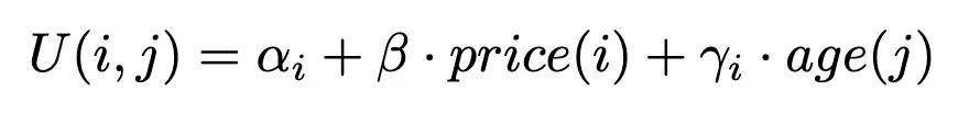
This function represents the utility (or satisfaction) a customer derives from choosing a particular item, influenced by both the customer’s age and the item’s price.
For more details on how we formulate a utility function, refer to our first post. Note that another logical — but not presented to keep it simple — model could be to estimate one price sensitivity per age category.
Here is the code to estimate such a model with choice-learn:
model.add_coefficients(
coefficient_name=age_category, feature_name=age_category, items_indexes=list(range(20))
)
coefficient_name=“price”, feature_name=“SALES_PRICE”, items_indexes=list(range(20))
)
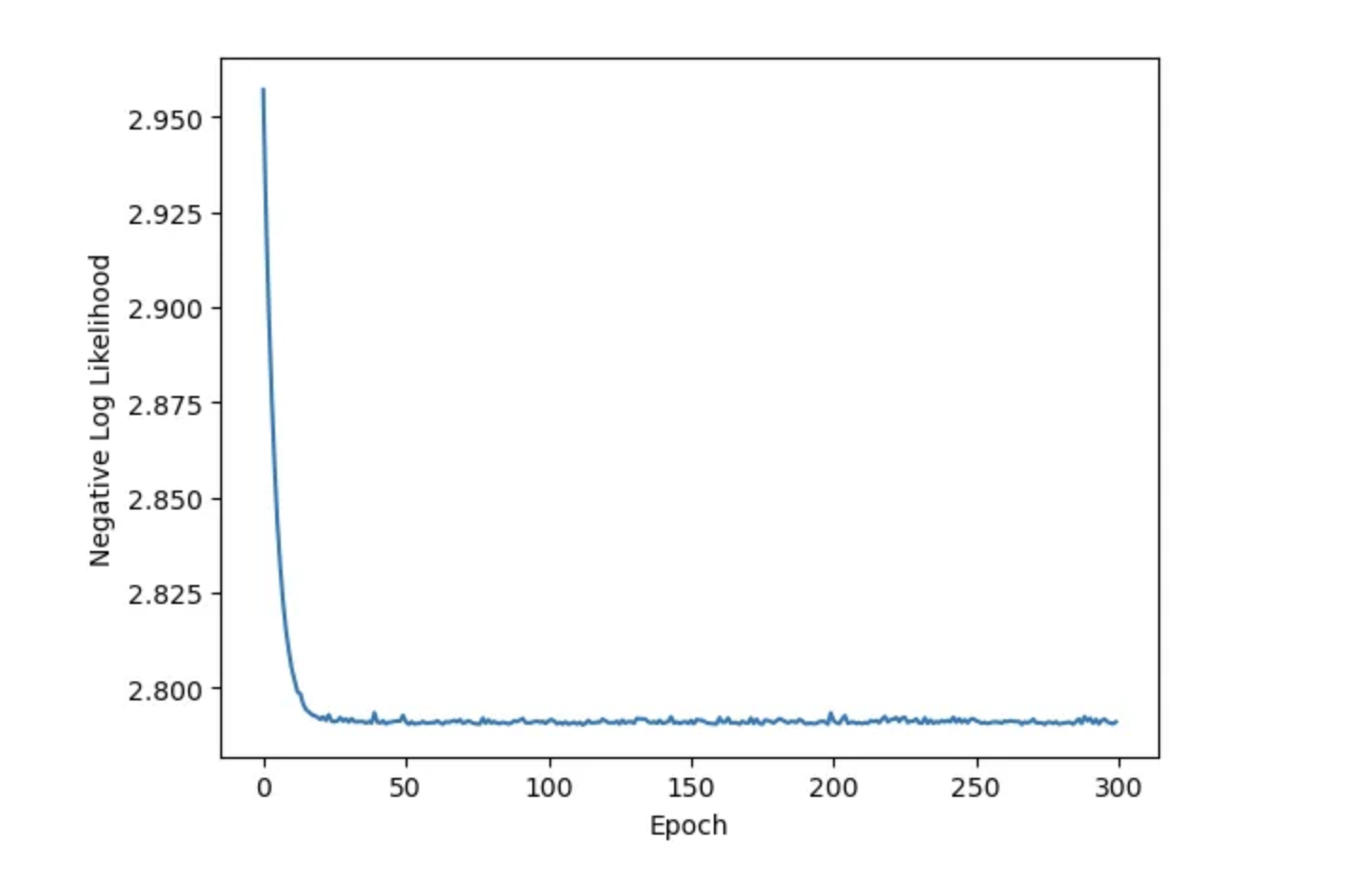
You can check that the model does fit well on the dataset:
plt.plot(hist[“train_loss”])
plt.xlabel(“Epoch”)
plt.ylabel(“Negative Log Likelihood”)
plt.show(
Finding the optimal assortment
With the purchase probabilities in hand, we can now estimate the average revenue per customer of an assortment A using the formula:

To find the assortment that maximizes revenue, we could evaluate all possible combinations and select the one with the highest average revenue. However, a more efficient approach is to use Linear Programming (LP). Here, we’ll focus on how to use the choice-learn implementation of the assortment optimizer.
It’s important to distinguish between maximizing revenue and maximizing profit margins. While revenue is important, profit margins take into account the costs associated with each product. Depending on your goal, you may want to optimize for profit rather than pure revenue.
To optimize the assortment, we need to provide several key inputs:
- The weight we want to give to each age category, let’s go with their customer share
- The utility of each item (calculated by our choice model) for each age category
- The value to optimize for each item (in this case, revenue)
- The size of the assortment (for example, 12 items)
Here’s how it works using choice-learn:
from choice_learn.toolbox.assortment_optimizer import LatentClassAssortmentOptimizer
# Price of each item
future_prices = np.stack([items_features[-1]]*5, axis=0)
age_category = np.eye(5).astype("float32")
# Compute utility of each item given its price and each age category
predicted_utilities = model.compute_batch_utility(shared_features_by_choice=age_category,
                                                  items_features_by_choice=future_prices,
                                                  available_items_by_choice=np.ones((5, 20)),
                                                  choices=None
                                                  )
age_category_weights = np.sum(shared_features, axis=0) / len(shared_features)
opt = LatentClassAssortmentOptimizer(
solver="or-tools", # Solver to use, either "or-tools" or "gurobi" (if you have a license)
class_weights=age_category_weights, # Weights of each class
class_utilities=np.exp(predicted_utilities), # utilities in the shape (n_classes, n_items)
itemwise_values=future_prices[0][:, 0], # Values to optimize for each item, here price that is used to compute turnover
assortment_size=12) # Size of the assortment we want
assortment, opt_obj = opt.solve()
Running the code you should have something like:
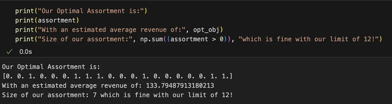
The optimal assortment for maximizing revenue is indicated with the indexes of the 1 values in the vector. This assortment theoretically yields an average revenue per customer of 134 yuan. You can explore other combinations, but they will all result in lower average revenue.
Another objective could be to maximize the number of sales. In this scenario, the item-wise value for optimization is set to 1 for all items, leading to a different optimal assortment.
The efficiency of this method becomes evident when additional constraints are introduced. For instance, you may need to account for shelf space limitations in your store. In this case, you can optimize for an assortment whose total item size does not exceed the available shelf space. This additional constraint, along with others such as pricing strategies, is demonstrated here.
Conclusion
If you are working on assortment optimization or pricing, choice modeling is a great tool, be sure to look into it. Choice-Learn provides many cool examples on its GitHub. Go check it out and leave as star if you find it useful !